Did the Minimum Wage Reduce the Gender Wage Gap in Germany?

DISCUSSION PAPER SERIES

IZA DP No. 14926

Marco Caliendo

Linda Wittbrodt

Did the Minimum Wage Reduce the

Gender Wage Gap in Germany?

DECEMBER 2021

Any opinions expressed in this paper are those of the author(s) and not those of IZA. Research published in this series may

include views on policy, but IZA takes no institutional policy positions. The IZA research network is committed to the IZA

Guiding Principles of Research Integrity.

The IZA Institute of Labor Economics is an independent economic research institute that conducts research in labor economics

and offers evidence-based policy advice on labor market issues. Supported by the Deutsche Post Foundation, IZA runs the

world’s largest network of economists, whose research aims to provide answers to the global labor market challenges of our

time. Our key objective is to build bridges between academic research, policymakers and society.

IZA Discussion Papers often represent preliminary work and are circulated to encourage discussion. Citation of such a paper

should account for its provisional character. A revised version may be available directly from the author.

Schaumburg-Lippe-Straße 5–9

53113 Bonn, Germany

Phone: +49-228-3894-0

Email: [email protected] www.iza.org

IZA – Institute of Labor Economics

DISCUSSION PAPER SERIES

ISSN: 2365-9793

IZA DP No. 14926

Did the Minimum Wage Reduce the

Gender Wage Gap in Germany?

DECEMBER 2021

Marco Caliendo

University of Potsdam, IZA, DIW and IAB

Linda Wittbrodt

University of Potsdam

ABSTRACT

IZA DP No. 14926 DECEMBER 2021

Did the Minimum Wage Reduce the

Gender Wage Gap in Germany?

In many countries, women are over-represented among low-wage employees, which is why

a wage floor could benefit them particularly. Following this notion, we analyse the impact

of the German minimum wage introduction in 2015 on the gender wage gap. Germany

poses an interesting case study in this context, since it has a rather high gender wage

gap and set the minimum wage at a relatively high level, affecting more than four million

employees. Based on individual data from the Structure of Earnings Survey, containing

information for over one million employees working in 60,000 firms, we use a difference-

in-difference framework that exploits regional differences in the bite of the minimum wage.

We find a significant negative effect of the minimum wage on the regional gender wage

gap. Between 2014 and 2018, the gap at the 10th percentile of the wage distribution was

reduced by 4.6 percentage points (or 32%) in regions that were strongly affected by the

minimum wage compared to less affected regions. For the gap at the 25th percentile, the

effect still amounted to -18%, while for the mean it was smaller (-11%) and not particularly

robust. We thus find that the minimum wage can indeed reduce gender wage disparities.

While the effect is highest for the low-paid, it also reaches up into higher parts of the wage

distribution.

JEL Classification: J16, J31, J38, J71

Keywords: minimum wage, gender wage gap, regional bite

Corresponding author:

Marco Caliendo

University of Potsdam

Chair of Empirical Economics

August-Bebel-Str. 89

14482 Potsdam

Germany

E-mail: [email protected]

* The authors thank Alexandra Fedorets, Cosima Obst, Stefan Tübbicke, and participants of the Annual Conference

of ESPE (Antwerp, 2018), the Annual Conference of EALE (Lyon, 2018) and the Potsdam Research Seminar in

Economics (Potsdam, 2021) for helpful discussions and valuable comments. We further thank the Federal Statistical

Ofﬁce and the statistical ofﬁces of the Länder for their help in supplying the data.

1 Introduction

The di↵erences between men’s and women’s earnings have been studied exte ns i vely over

recent years. One of its dimensions is the fact that women are often overrepresented among

the low-paid employees (Kahn, 2015; Card et al., 2016). This leads to the existence of a

wage gap at the bottom of the distri bu t i on, also called ‘sticky ﬂoors’, and one possible way

to alleviate t h i s issue is the introduction of a minimum wage. If female employees are more

prevalent among the wage ﬂoor beneﬁciaries than their male counterparts, they should also

be disproportionately a↵ected by a minimum wage, which would reduce wage disparities and

thus the gender wage gap. In their seminal paper, DiNardo et al. (1996) ﬁnd that labour

market institutions such as a minimum wage can indeed reduce inequality, especially so for

women. This line of research has been continued by an ample number of studies establishing

a negative relationship between the minimum wage and the gender wage gap for a variety of

countries.

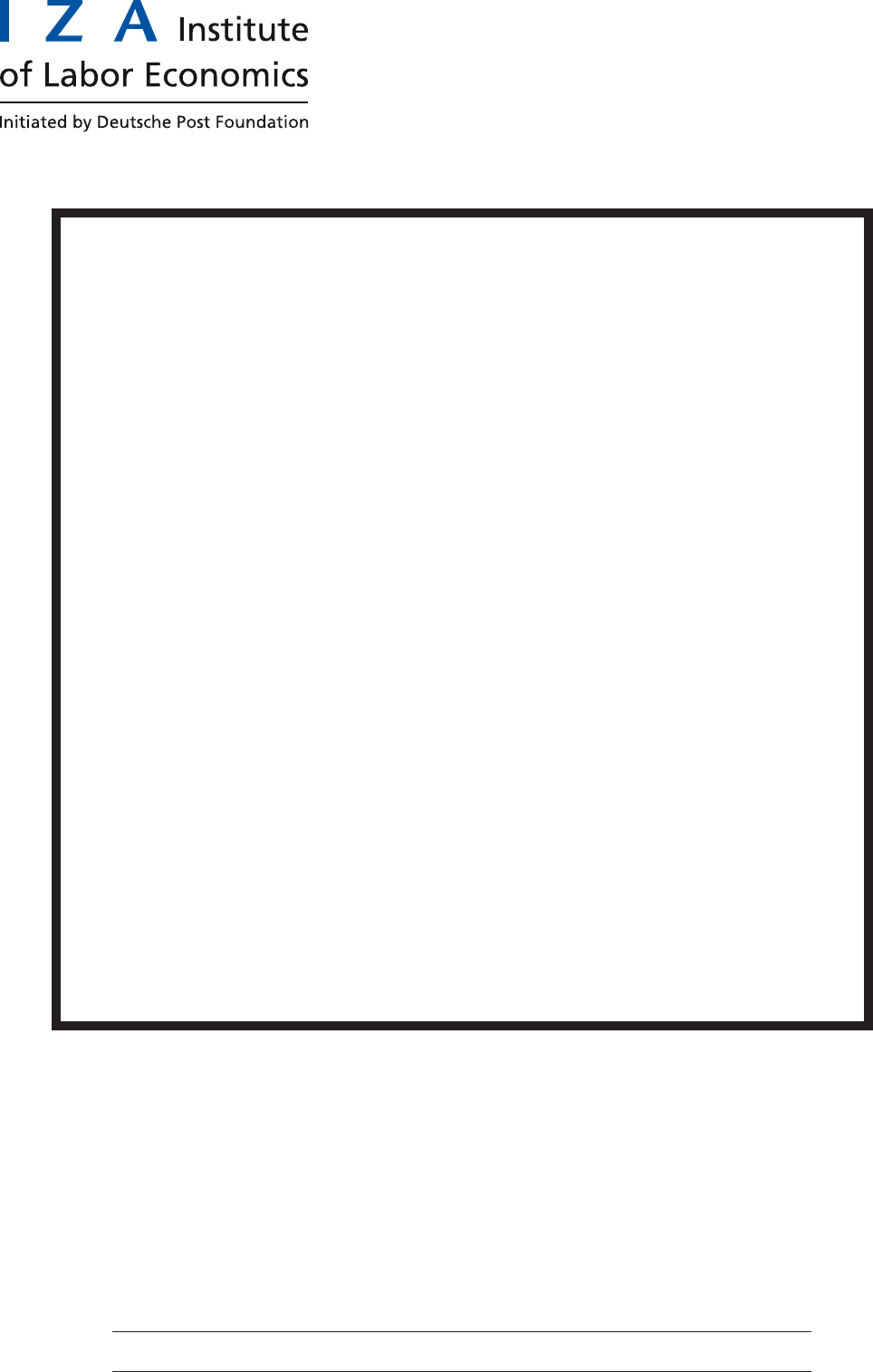
In this context, Germany poses an interesting case study. On the one hand, it i s a country

with a relatively high gender wage gap, especially at the bottom of the wage distribution. In

2014, the di↵erence between the earnings of full-time employed men and full-time employed

women amounted to 17.2 percent in Germany, placing it in the upper third of countries with

the highest gaps, above the OECD average (see Figure 1a).

At the ﬁrst decile of the wage

distribution, Germany even shows a wage di↵erence of 18.2% in 2014, placing i t among the

eight countries with the highest gaps among low-income earners, and well above the United

States and t h e United Kingdom (see Figure 1b). It is thus evident that Germany su↵ers from

high gender wage discrepancies in an OECD comparison, especially among low-wage earners.

On the other hand, Germany introduced a nationwide minimum wage in 2015, which was

set at a comparably high level and had only few exemptions.

With e8.50 gross per hour,

it ranked among the highest wage ﬂoors in Europe in terms of purchasing power (Caliendo

et al., 2019). Its level is to be re-eval u at ed every two years, and it was increased to e8. 84

See for example Bargain et al. (2019)andRobinson (2005) for UK and Ireland, Broadway and Wilkins

(2017) for Australia, (Hallward-Driemeier et al., 2017) for Indonesia, Li and Ma (2015) for China, and Ma -

jchrowska and Strawinski (2017) for Poland.

In this paper, we look at the unadjusted wage gap, also call ed the raw gap. A substantial part of the raw

gap can be explained by observable factors, such as di↵erences in schooling, working hours, etc. For Germany,

these factors can explain around three quarters of the gap (Destatis, 2020). The remaining unexplained part

is called adjusted gap.

The law only stipulat ed a few exemptions, mainly minors, trainees, speciﬁc interns, volunteers and long-

term unemployed. Additionally, employees in sectors with pre-existing wage ﬂoors below e8.50 were exempted

until the end of 2016 (for details, see also Caliendo et al., 2019). For the Minimum Wage Act, see https:

//www.gesetze-im-internet.de/englisch_milog/index.html,lastaccessedonNovember11,2021.

in January 2017, being followed by additional increases in 2019 and the subse qu ent years

(Mindestlohnkommission, 2016a, 2018, 2020a). Caused by its high initial value, the reform

a↵ected about four mill ion employees, i.e. about ten percent of the eligible workers (Destati s,

2016). Among them, women were vastly overrepresented, since they accounted for two-thirds

of a↵ected employees ( Mi nd es t loh n kommission, 2016b; Burauel et al., 2017). This has been

attributed to insuﬃcient regulations of the low-pay sector and gender segregation, which lead

to an unequal coverage of collective bargaining agreements for men and women (Grimshaw

and Rubery, 2013; Herzog-Stein et al., 2018). Accordingly, the i ntro d uc t ion of t h e wage ﬂoor

could have an inﬂuence on gender inequality. In a simulation study for Germany, Boll et al.

(2015) predict that in the absence of job losses, the minimum wage could reduce the average

gender wage gap by 2.5 percentage points. However, with job losses, the e↵ect could even be

larger. This points to a potential caveat, namely that low-paid women quitting or losing their

jobs would cause a decrease in the gap. However, since ex-post evaluation studies on Germany

ﬁnd only s mal l empl oyment e↵ects and no strong evidence of gender-speciﬁc job-losses, we

assume that there are no signiﬁcant heterogeneous employment e↵ects (see Caliendo et al.,

2019; Bonin et al., 2018; Pestel et al., 2020).

In our analysis, we mainly employ data from 2014 and 2018, which we obtain from the

Structure of Earnings Survey (SES), a large obligatory survey that comprises de t ai le d wage

information for over one million employees working in 60,000 ﬁrms. First, we des cr i pt i vely

look at the wages of male and female employees who are eligibl e for the minimum wage

and compare the wage gap in 2014 with the one i n 2018. Second, following Card (1992),

we make use of regional variation in the “minimum wage bite”, i.e. the degree to which a

region is a↵ected by the minimum wage, and analyse the causal e↵ects of the minimum wage

introduction on regional gender wage gaps.

We are able t o identify a signiﬁcant e↵ect on

the wage gap at the regional level, especially for low-paid e mp loyees. Between 2014 and 2018,

the gap at the 10

percentile was reduced by 4.6 percentage points (or 32%) in regions that

were strongly a↵ect ed by the minimum wage compared to less a↵ected regions. For the gap

at the 25

percentile, the e↵ect still amounted to -18%, while for the mean it was smaller

(-11%) and not particularly robust. Using a continuous bite measure, we can show that an

increase in a region’s bite by ten p er c entage points, reduce s the wage at the 10

percentile

Since our po st -re fo rm data is from 2018, in our analysis we estimate the e↵ect of b o th the initial intro-

duction of the minimum wage as well t h e ﬁrst increase from 2017. However, p rev io u s research shows that

the reform had mainly signiﬁcant wage e↵ects in 2015, whereas th e re were no relevant e↵ects after the ﬁrst

increase in 2017 (Burauel et al., 2020; Fedorets et al., 2019).

by 3.3 percentage points. This thus shows that the minimum wage reform led to a signiﬁcant

decrease in the wage gap especially at the bottom of the wage distribution.

The remainde r of this paper proceeds as foll ows. Section 2 reviews the previous literatur e

on gender-speciﬁc minimum wage e↵ects on wages and presents the data that we use. Addi-

tionally, it o↵ers a ﬁrst descript ive overview of the gender-speciﬁc wages before and after the

reform, as well as the regional d i↵ er en ce s in the wage gap and the bite measure. Section 3

then presents the identiﬁcation strategy and d i sp lays the results of the main estimation and

the robustness analyses. In section 4, we summarise our results.

2 Previous Evidence, Data and Descriptives

2.1 Previous Evidence

The previous evidence on gen d er -speciﬁc wage e↵ects of the German minimum wage is scarce.

In a descriptive analysis with the Socio-Economic Panel (SOEP), Herzog-Stein et al. ( 2018)

ﬁnd that the wage gap at the te nth percentile had reduced by seven percentage poi nts (from

22% to 15%) two years after the reform, which the authors attri bu t e to the minimum wage.

Interestingly, the gender gap stagnated for the lowest paid ﬁve percent (at 18%), which they

relate to circumvention strategies. Ohlert (2018) looks at wages below e10 in 2014 and 2015

and ﬁnds that women’s wages increased more strongly (14.6%) than men’s wages (11.3%)

in East G er many, while in the former West German states there was no gender-speciﬁc

di↵erence.

Additionally, some causal s t ud i es on wage e↵ects h ave included some gender-

speciﬁc heterogeneity analyses. However, they do not estim ate the e↵ect on t he wage gap

itself and su↵er from small samples sizes. Burauel et al. (2018) ﬁn d t h at between 2014 and

2016 the minimum wage e↵ect on hourly wages was signiﬁcant for women and amounted to

about 5.9%. While the male e↵ect was larger, it did not satisfy the common trend assumption,

challenging the results for this subgroup. Bachmann et al. (2020) ﬁnd that female employees

earning less than e8.50 in 2014 experienced a statistically signiﬁcant wage growth of 5.7%

directly after th e reform, while the e↵ect for men was postponed: they beneﬁted from a wage

growth of about 10.2% from 2015 to 2016 and 14.8% in the following year. There was no su ch

e↵ect on women’s wages at this time. Overall, previous stu di e s ﬁ nd i nd i cat i ons t hat wages

However, th e results are based on the voluntary Earnings Survey (ES) and are potentially inﬂuenced by

selectivity issues (see Ohlert, 2018; D¨utsch et al., 2017).

among the low-paid employees rose due to the minimum wage introduction.

Moreover, there

is evidence that women’s wages rose more strongly s hor t l y after the r e for m and men’s e ↵ect s

were possibly postponed. However, none of these studies have explicitly examined the e↵ects

of the minimum wage on the gender wage gap.

2.2 Data Source s and Preparation

There are only a few datasets that are suitable for evaluating the minimum wage e↵ects in

Germany. All of them have di↵erent advantages but also caveats and neither is completely

ideal. The di↵erences as well as the associated issues have been widely discussed before (see,

e.g., Caliendo et al., 2019; Mindestl ohn kommission, 2020b). In this paper, we rely on the

SES

, provided by the Federal Statistical Oﬃce of Germany (Destatis). It is a rich earn i ngs

survey in which employers are obligated to participate. Next to ﬁrm level data, t h e SES entails

detailed individual information taken directly from payroll accounting or p e rs onne l statistics.

It has ﬁrst been collected in 1951 and takes place every four years since 2006. In this paper,

we mainly make use of the most direct pre- and post-reform waves that are available, namely

2014 and 2018. Additionally, we look at the dat a from 2010 in Section 3.3 in order to check

the pre-treatment trends.

The SES 2014 and 2018 are well suited for our analysis since they are large datasets, that

each contain more than 1 million employees working in ove r 60,000 ﬁrm s. The businesses

were obliged to provide information on wages, working hours, and other working condit i ons ,

allowing us to construct precise hourly wages. However, two caveats should also be noted. First

of all, it does not take place yearly, forcing us to look at a rather long time-frame. Second, it

is not a panel study but largely comprises re peated cross sections. The recent waves include

employees from nearly all economic sectors that have at least one employee. Nonetheless,

we exclude public sector employees, since for them there is no detailed regional information

available beyond the federal state. However, since this sector does not typically su↵er from

low wages, it is not strongly a↵ected by the minimum wage. The SES is representative at the

level of the sixteen federal states. In order to exploit the regional variation of the minimum

wage bite, we follow previous studies (see for example Bachmann et al., 2020) and rely on

the smaller 257 labour market region s (“Arbeitsmarktregionen”). Moreover, in a sensitivity

See also Ah lfe ld t et al. (2018), w h o ﬁnd that wages in low-wage counties increased more rapidly than in

high-wage counties, particularly so for low-paid employees.

Source: FDZ der Statistischen

Amter des B u n d es und der L¨ander, Verdienststrukturerhebu n g , 2010, 2014

and 2018.

analysis we also look at planning regions (“Raumordnungsregionen”) and districts (“Kreise

und kreisfreie St¨adte”), the former being a less and the latter a more disaggregated regional

classiﬁcation (see Section 3.4).

Since the SES does not collect data on hourly wages, we compute them using monthly

income and working hou r s. We employ the gross month l y earnings and subtract earnings

received for premiums and overtime worked. We divide this by the number of paid working

hours (ex cl u di n g ove rt i me ) .

In our analysis, we only look at employees who are eligible for

the minimum wage. We thus ex cl ud e trainees, interns as well as minors without a vocational

training.

We generate the gender wage gap at the regional level as the di↵erence between

men’s and women’s wages divided by men’s wages. We do this for regional mean wages but

also wit h the wages at the 10

and 25

percentiles of the gender-speciﬁc wage distributions.

This allows us to look at wage di↵erences not only at the mean but also speciﬁcally among

low-paid employees.

2.3 Descriptive Statistics

Wage Gap and Fraction of A↵ected Employees As a ﬁrst step in our empirical anal-

ysis, we examine di↵erent aspects of the gend er wage gap descriptively.

As shown in Table

1, we rely on inform at i on for 755,431 individuals in 2014, 46% of th em being female. In 2018,

there are 742,716 individuals included, 44.9% of which are women. The mean wage of em-

ployees in our sample amounted to e16.80 in 2014. While me n eligible for the minimum wage

earned about e19.0 on average, their female counterparts earned only e14. 4. This translates

into a gender wage gap of 24.5%.

Four years later, wages had increas ed overal l, but women’s

wages more strongly. Consistently, the wage gap at the mean decreased to 21.9% in 2018.

[Insert Table 1 here]

If the number of paid working hours is not known, we divi d e by regular weekly working hours times 4.33,

which is the average number of weeks in a month.

Since we cannot identify employees working in sectors with pre-existing wage ﬂ oors below e8.50, we follow

previous studies and include them in our analysis (see e.g., Ohlert, 2018). This should not a↵ect our results

as these were only few sectors and regulations ran out at the end of 2016 (Mindestlohnkommission, 2016b).

Nevertheless, we will address this issue in our robustness analysis.

The SES provides individual weights that we use for the general descriptives and the calculation of regional

wages an d wage distributions. While the weights yield representative results on the level of federal states, they

do not necessarily do so for a sm a ll er regional level (s ee FDZ der Statistischen

Amter des Bundes und der

L¨ander, 2019, for details). Therefore we exclude the weights as a sensitivtiy check in S ec ti o n 3.4.

It should be noted that the gender wage gap in our sample is la rg er than that for the overall population

found in other studies. This is caused by di↵erent factors. First, we do not include public sect o r personnel,

whose inclu sio n would lead to th e gap being sma l ler. Second, we only look at workers who are not exempt from

the minimum wage. Finally, we focus on the raw/unadjusted gender wage gap, while many studies examine

the (lower) adjusted gap.

It al so becomes apparent that women were overrepresented in the low-wage sector. In

2014, 9.3% of men but 16.3% of women were earning less than e8.50 per hour. Looking at

the ﬁrst minimum wage increase to e8.84, nearly every ﬁfth woman (19.8%) in our sample was

a↵ected in 2014, compared with only 11.5% of me n. Four years later, i.e. after the introd uc t i on

and ﬁrst increase of the minimum wage, less th an one percent of either gender earne d less than

e8.50 and 2.8% of employees earned le ss than e8.84. However, among women the percentage

was slightly larger than among men, suggesti ng that women were disproportionately a↵ected

by non-compliance with the wage ﬂoor.

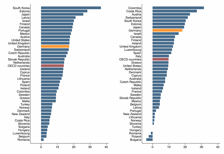
Wage Gap Over the D is tri b u tion Our sample displays a higher wage gap at the top of

the wage distribution: in 2014, it amounted to 31% at the 90

percentile, but to only about

10% at the ﬁrst decile. However, the largest decrease in the gap is found at the bottom: at the

percentile, the gap decreased by 3.84 per ce ntage points. A more detailed representation

of this is displayed in F igu r e 2. Here, we depict the wage gap at twenty quantiles. Between

2014 and 2018, th e gap decreased along the whole distribution, but especial l y up to the 15

percentile. Remembering that 16.3% (19.8%) of women earned less th an e8.50 (e8.84) in

2014, this indicates a connection to the min imum wage introduction. The strongest reduction

took place at the ﬁ f t h per ce ntile, where the gender wage gap in h ou rl y wages decreased from

8.5% to 1.3% among eligible employees in our sample. There was also a strong reduction in

the gap at the 10

and 15

percentile. However, at the 20

and 25

percentiles – i.e. above

the share of a↵ected women – it remained nearly constant.

[Insert Figure 2 here]

Regional Variation and Development Our ﬁndings are also underlined by Figur e 3,

which displays the regional variation in the gender wage gap at the ﬁrst decile, i.e. one of the

dependent variables in our later analysis. Figure 3a and 3b map the gap in 2014 and 2018,

where red colouring indicates a positive wage gap and blue colouring a negative gap. The

higher the absolute value, the higher t h e colour intensity. F i gur e 3c displays the di↵erence

in the gap between the two years.

It highlights the fact that the gap among th e low-

All evaluations of (non-)compliance ﬁnd that a substantial number of eligible workers were paid less than

the minimum wage even after the reform. Estimations of the magnitude of that issue di↵er depending on the

data source. Summarising a number of studies, the minimum wage commission plac es non-compliance in the

range of 1.3% to 6.8% for 2018 (Mindestlohnkommission, 2020b).

Note that in the regional descriptives, information for Saxony is averaged over all Saxon labour market

regions due to data ap p roval issues. However, in our later analysis, we use detailed data on the ten Saxon

regions.

paid decreased from 2014 to 2018 in most regions. Addi t i on all y, we see that in the East of

Germany, the picture is rather homogeneous: the gap at the 10

percentile was reduced in all

East German regions, in many of them between ﬁve and ﬁfteen percentage points. However,

in the West, the development is more diverse. There are some re gion s that experienced a

strong decrease in the gap, but also regions in which the gap substantially increased.

[Insert Figure 3 here]

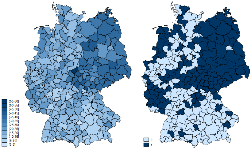
The Minimum Wage Bite Another variable central for our analysis is the minimum wage

bite, measuring the degree to which a region was a↵ected by the minimum wage in 2014. The

literature features a variety of b it e measures such as the fraction of a↵ected employees or

the Kaitz index (see al so Caliendo et al., 2018). However, the Kaitz index indicates th e ratio

between th e minimum wage and the regional mean wage and it is thus also a↵ect e d by other

determinants of the mean wage, which is why we focu s on the fraction of a↵ected employees.

More precisely, we employ the regional share of el i gi bl e women earn i ng less than the wage

ﬂoor in relation to all eligible women (henceforth called ‘fraction’), since we aim t o identify

regions in which women were especially a↵ected by the minimum wage. Figure 4a displays

the fraction for the 257 labour market regions in 2014. It can be seen that – in contrast to

the wage gap – the bite is generally higher in the East of Ge rm any. However, there are also

regions in the West where women are a↵ected above average. For the empirical analys i s later

on, we will use a binary “high-bite” indi cat or and spl it t h e sampl e into high- and low-bite

regions at the median bite level of 17.15%. Figure 4b shows the regional distribut i on of this

new indicator. While all regions in East Germany are high-bite regions (equal or above the

median) and receive a value of 1 for this indicator, it also bec ome s clear that high-bite regions

are found across the whole country.

[Insert Figure 4 here]

3 Methodological Approach and Results

3.1 Empirical Approach

In this paper, we aim to identify the impact of the German minimum wage on the gende r wage

gap. In our identiﬁcation strategy, we follow Card (1992), who proposes an approach relying

on regional variation (also employed by other authors, e.g. Stewart, 2002; Dolton et al., 2010,

2012, 2015; Caliendo et al., 2018). In contrast to other methods, it t he r ef ore does not depend

on di↵erences in legislat i on, which do not occur in the German case (see also Cal ie nd o et al.,

2018). The approach incorp orat e s the intuition that r e gion al wages have to adapt to varying

degrees in accordance with the introduction of a minimum wage. In regions where wages

were lower prior to th e introduc ti on , the minimum wage is assumed to bite harder into the

wage distribution and its e↵ect on potential outcomes is thus expe ct ed to be stronger. The

corresponding ﬁxed e↵ects estimation equation of the gender wage gap is deﬁned as follows:

Gap

j,t

= ↵

+ T

2018

+ T

2018

Bite

2014

+ X

j,t

+ 

j,t

,witht= {2014, 2018} (1)

where Gap

j,t

denotes the gender wage gap in percent in region j at time t. ↵

is a region-

ﬁxed e↵ect and T

2018

is a dummy taking the value of 1 in the year 2018. X

j,t

is a set of

regional controls an d 

j,t

is the error ter m. Bite

2014

denotes the regional bite. While we use

the fraction of a↵ected women in our main analysis, we also make use of the fraction of

a↵ected employees over both genders in our sensitivity anal y si s . In order to obtain a clearer

picture, we employ the fraction as a binary bite measur e , dividing regions at the median

fraction. In t h e robustness checks, we also include t he fraction as a continuous variable. X

j,t

entails control variables provided by the INKAR database.

It comprises of the regional

GDP per capita, the popul at i on density, t h e share of women, the female employment rat e

as well as the uptake of childcare f or children under three and children between t h re e and

ﬁve. All of those are m easu r ed in the prev i ous year to avoid endogeneity issues.

To control

for time persistent regional characteristics, we employ a ﬁxed e↵ect estimation with robust

standard errors.

The identifying assumption of the di↵erence-in-di↵ere nc e approach that we emp loy is that

the treatment regions (i.e. high -b i t e regions) and control regions (i.e. low-bite regions) have

common trends in the wage gap in the absence of the treatment. In order to test this, we

estimate a placebo regression in Section 3.3, assuring us that the common trend assumption

holds. However, we ﬁrst turn to our main results in the following section.

The “Indicators, Maps and Graphics on Spatial and Urban Monitoring” d a t ab a s e is provided by the

Federal Institute for Research on Building, Urban A↵airs and Spatial Development (BBSR Bonn, 2021).

The control variables are precisely deﬁned as follows: gross domestic product in e1,000 per inhabitant,

inhabitants per km

, the share of women among inhabitants i n percent, the s h a re of women with contracts

subjec t to socia l security contributions among all women in working age, the share of children under three

years in childcare among all children under three, the share of children between three and six years in childcare

among all children between three and six.

3.2 Main Result s

In our main analy si s we estimate equation (1) described in Secti on 3.1 with ﬁxed e↵ects.

As already done in Section 2.3, we look at the wage gap at three di↵erent points of the

distribution: the 10

and the 25

percentile as well as th e mean. Accordingly, ou r results

are divided with respect to these outcome variables, which is indicated by the t hr ee di↵erent

panels in Table 2. Within each panel, we include the control variables in six steps, captured

by columns (1) to (6). The table shows the coeﬃcients and indicates their signi ﬁc anc e.

[Insert Table 2 here]

The ﬁrst panel estimates the e↵ect on the gap at the tenth percentile. Without the

inclusion of further control variables (column 1), there is a strongl y signiﬁcant treatm e nt

e↵ect of -5.2 percentage points. This is to say that – in comparison to regions wit h a low bite

in 2014 – hi gh- bi t e regions experi en ce a reduction of the wage gap at the tenth percentile of

5.2 percentage points in 2018, ceteris paribus. This is accompanied by a general reduction

of the gap of 3.6 percentage points between 2014 and 2018. When we include additional

control variables iteratively, the magnitude of the treatment e↵ect only slightly decreases and

the signiﬁcance is unchanged. In the most comprehensive speciﬁcation (column 6), high-bite

regions experience a reduction in the wage gap of 4.6 percentage points from 2014 to 2018

due to the minimum wage. This corresponds to a reduction of about 32% in the wage gap

(compared to the level in 2014 which was 14.4% in these regions). It is interesting to note,

that the signiﬁcance of the dummy for 2018 vanishes after controlling for the employment

rate of women, meaning that the wage gap for low-paid employees only reduced for highly

a↵ected regions, and very strongly so. When look i ng at the wage gap at the 25

percentile

(see Panel B), the treatment e↵ect is still highly signiﬁcant but not as large. It ranges from

-2.8 to -3.4 percentage points depending on the speciﬁcation. In our preferred speci ﬁ cat i on

(column 6) it corresponds to a relative e↵ect of -18% compar ed to the level in 2014 ( whi ch

was at 18.3%). For the wage gap at the mean (Panel C), the e↵ects are least pronounced:

in the most comprehensive speciﬁcation (column 6), t h e signiﬁcant treatment e↵ect amounts

to -2.3 per ce ntage points, correspondi n g to a relative reduction of 11% (compared to the

2014 level which was 20.4%) . The results suggest that there was a general reduction of the

wage gap at the mean between 2014 and 2018, but regions in which women were particularly

a↵ected by the minimum wage exper i en ce d an additional decre ase.

Overall, the analys i s shows that there is a strong e↵ect of th e minimum wage, which is

especially large at the bottom of the wage distribution. The gap at the tenth percentile is

reduced by 4.6 percentage points (32%) between 2014 and 2018 in regions that were strongly

a↵ected by the minimum wage compared with less a↵ect ed regions. Higher up in the distri-

bution, the magnit u de and signiﬁcance of the results decrease. However, an e↵ect can still be

detected and it ranges from 18% at the 25

percentile to 11% at the mean.

3.3 Common Trend

In order to analyse the common trend assumption, we make use of the 2010 wave of the

SES. However, the structure of the SES signiﬁcantly chan ged between 2010 and 2014. In

2010, there were fewer sectors included and – most important to our case – there were no

ﬁrms with fe wer than ten employees subject to social security contributions. Additionall y, the

month of data collection changed. Overall, there is information on over 1.9 mil li on employees

in about 34,000 businesses included in 2010, in comparison to about one million workers

in 60,000 busi n ess es in 2014 (Destatis, 2013; FDZ der Statistischen

Amter des Bundes und

der L¨ander, 2019). Therefore, given that we cannot simply compare our previous results to

the 2010 data, we make use of a subsample of ﬁrms, which we identify via a variable that

is provided by the federal statistical oﬃce and that adapts the 2014 and 2018 data to the

structure of the 2010 wave (FDZ der St at i st i schen

Amter des Bundes und der L¨ande r, 2019).

This leads to a slightly di↵ er ent subsample in comparison to our main analysis (see Table

A.1): here, a smaller share of male and female employees was a↵ect e d by the introduction

of the wage ﬂoor. Accordingly, the wages that they display are higher. One reason for this

is that the su bs amp l e does not include ﬁrms with fewer than ten employees, which usually

pay less. Additionally, the gender wage gaps are slightly di↵erent between the two sampl es.

However, the two samples are comparable overall.

In Table 3 we show the results of re-running the equation 1 with our subsample (columns

4 to 6) as well as the equation adapted to the pre-reform period (columns 1-3), which is

deﬁned as follows:

Gap

j,t

= ↵

+ T

2014

+ T

2014

Bite

2014

+ X

j,t

+ 

j,t

,witht= {2010, 2014} (2)

The table shows that when looking at the time before the minimum wage introduction, i.e.

between 2010 and 2014, the wage gap evolved similarly in high- and low-bite regions, which

is in di cat e d by a statistically insign iﬁ cant interaction term. This conﬁrms our assumption of

a common trend in the gap before the reform. When turning to the replication of our main

regressions for the years 2014 and 2018 with the subsamp l e, we observe very similar results

to our main speciﬁcati on presented in Section 3.2. Agai n , we ﬁnd signiﬁcant e↵ects for the

and 25

percentile that are also comparable in magnitude. However, in contrast to our

main resu lt s in Table 2, we do not ﬁnd a signiﬁcant e↵ect for the mean gap. Nonethe le ss , our

results give us conﬁdence that the common trend holds and that the wage gaps would have

developed si mi l arly in high- and low-bite regions in absence of the reform, especially for the

lower parts of the distribution.

[Insert Table 3 here]

3.4 Robustness Analysis

In the following, we will test the sensitivity of our results to a number of pract i cal implemen-

tation issues. We lo ok at di↵erent computations of the minimum wage bite, the e xc l us ion of

employees working in sectors with sector-speciﬁ c minimum wages, di ↵e re nt regional classiﬁ-

cations, a non-weighted bite measure and weighted labour market regions.

Di↵erent Bite Measures First, we employ other variations of the bite measure. As dis-

cussed in Section 2.2, our mai n analysis relies on the ratio of a↵ected female employees in

2014 to all female employees in 2014. However, we could also employ the minimum wage

bite for all employees, irres pective of their gender. We thus re-run the estimation using the

overall fraction (see Panel B in Table A.2, Panel A repeat s the results of the main analysis for

comparison). The r es ul t s mirror those of the ful l estimation of our main an al ys i s, although

the e↵ects are not as large in magnitude. This is caused by the fact that the fraction of af-

fected employees calculated for women only better i d entiﬁes th e re gion s t hat are p art i cu l ar ly

subject t o reductions in the wage gap. However, regions where men are also highly a↵ect ed

are not ex pected to experience a pronounced decrease in the wage discrepancies. A second

bite variation that we employ is the continuous bite (see ﬁrst Panel C in Table A.2). In our

main estimation, we only distinguished between low-bite and high-bite regions, cut o↵ at

the median bite. Now we include the f rac t i on of a↵ected female employees as a continuous

variable, allowing for more variation in the treatment. The variable ranges from 3.8% to

55.8%. Again, the structure of the results is rather similar to our mai n result s , although the

interpretation of the coeﬃcients is slightly di↵erent. Here, a ten-percentage-point increase in

the bite corresponds to a reduction of the wage gap at the tenth percentile by 3.3 percentage

points in 2018. Similarly, the gap at the mean decreases by 1.8 percentage points.

Excluding Sector-Speciﬁc Minimum Wages The law stipulates th at employees in sec-

tors with pre-existing minimum wages below e8.50 were ex em pt e d from the wage ﬂoor until

the end of 2016. Unfor t u nat el y, we are not able to identify these sectors in our data. Since

these were only few sectors and regulations ran ou t at the end of 2016, this should not a↵ect

our results. Nevertheless, in order to test the robsutness of our results in that directi on we

can exclu d e all employees subject to any sector-speciﬁc minimum wages (most of them were

above e8.50, see Mindestlohnkommission, 2016b, for more details) and re-run our estimation

(see Panel D in Tabl e A.2).

Again, the results are similar to the main estimat ion and do

not challenge our results.

Regional Classiﬁcations Moreover, we check the sensit iv ity in terms of the regional clas-

siﬁcation. In our main estimation, we decided to make use of the 257 labour market regions

since they supply more variation than the 96 planning regions and include more observations

per region th an the 401 districts. In order to check whether this decision inﬂuences our re-

sults, we now make use of these other regional divisions (see Panels E and F of Table A.2).

The results are very similar to our main results, although the e↵ects sizes are again slightly

smaller and the treatment e↵ect at the mean becomes insigniﬁcant. However, the e↵ects at

the 10

and 25

percentiles are robust and mostly highly signiﬁcant.

Weights Finally, we check whether our results are sensitive with respect to weighting is-

sues. First, we focus on the individual weights provided by the Federal Statistical Oﬃce.

As discussed before , our main analysis incorporates individual weights when calculating the

minimum wage bite and the region al wage distributions. However, these are designed to yiel d

representative res ult s on the level of federal states. Since we run estimation s on a smaller

regional level, we check whether the i nc l us ion of those weights inﬂuences ou r results. We

therefore re-run our estimation without them (see Panel G in Table A.2). Additionally, since

our main analysi s does not inc lu d e regression weights, we now repeat the analysis using the

regional employment in 2014 as esti mat i on weight s (see Panel H in Table A.2). The results of

both these sensitivity analyses are in line with the previous estimations, yielding very similar

We thus exclude 98,076 men and 79,654 women in 2014 and 94,602 men and 71,567 women in 2018.

results compared to our main regression.

Overall, our analyses conﬁrm the robust ne ss of our resu lt s for low-paid employees with

respect to di↵erent implementation decisions that we made in our main estimation. We can

thus conclude that there is a negative and highly signiﬁcant e↵ec t of the minimum wage on

the ge nd er wage gap at the bottom of the distribution. However, for the gap at the mean,

the results are not as robust.

4 Conclusion

The introduction of the minimum wage in Germany was a major intervention into the labour

market, which was – among other things – expected to reduce poverty and allevi at e inequality

(Bosch, 2007; Mindestlohnkommission, 2016b). One of the dimensions that could be a↵ected

is gender wage di↵erentials. Germany poses an interesting research case, since it exhibits both

large wage gaps and a high mi n i mum wage. In our paper, we have thus analysed whether

the wage ﬂoor did indeed lead to a decrease of the gender wage gap and – if so – at which

point(s) of the distribution. For this purpose, we employed a regional di ↵erence-in-di ↵ erence

approach, making use of the regional var iat i on in the degree to which female e mp loyees were

a↵ected by the minimum wage. Using comprehensive data from t h e Struc t ur e of Earnings

Survey, we identify regional wage gaps in 2014 and 2018 as well as the regional fraction of

a↵ected f emal e workers. Descri p t ively, we observe a reducti on in the wage gap between 2014

and 2018 for the whole distribution. However, we also see that it was particu l arl y reduced

among the low-paid employees.

In our di↵erence-in-di↵erence analysis, we ﬁnd that there was a signiﬁcant decrease in

the gender wage gap in regions in which women were strongly a↵ected by the minimum

wage in comparison t o regions where women were less a↵ected: high-bit e regions experienc e

a reduction of the wage gap at the 10

percentile of 4.6 per ce ntage poi nts from 2014 to 2018

due to the minimum wage, and this e↵ect is robust across speciﬁcations. The magnitude of

this e↵ect is large, corresponding to a relat ive reduction of about 32% compared to the level

in 2014. When looking at the bite in a continuous deﬁnition, we ﬁnd t h at increasing a region’s

bite by ten percentage points leads to a reduction of the wage gap at the 10

percentile by

3.3 percentage points. Our placebo estimations show that there was no such e↵ect before the

reform, i.e. that the common trend assumption is reasonable. Addit i on al ly, we ﬁnd that these

e↵ects fade out higher up the distribution. For the gap at the 25

percentile, the e↵ect still

amounted to -18%, while for the mean it was smaller (-11%) and not particularly robust.

Overall, our analysis suggests th at the mi n i mum wage can be an e↵ective tool for reducing

the ge nd er wage gap, especially at the lower end of the wage distribution. However, we do

not incorporate employment e↵ects. As discussed above, strongly a↵ected women could be

driven to quit or lose their jobs, which would artiﬁcially reduce the gender wage gap. While

previous studi e s do not ﬁnd st r ong evidence of this e↵ect, fut ur e research should focus on

this more thoroughly. Additionally, it would be insightful to determine the long-term e↵ects

on the gender wage di↵erentials. Thus far, we are re st r i ct ed to data fr om 2014 and 2018,

which al lows us to identify a medium-term e↵ect but neglects possible long-run adaptation

processes. Moreover, while our survey period includes the ﬁrst minimum wage increase, an

analysis of the subsequent raises could also yie ld relevant information. Fi nal l y, it would be

interesting to disentangle the e↵ects on the adjusted gender wage gap, not least because the

distinction between the two is often a very essential issue in the gender wage gap debate.

References

Ahlfeldt, G. M., Roth, D. and Se ide l, T. (2018) . The regional e↵ects of Ge rm any’s

national minimum wage. Economics Letters, 172, 127–130.

Bachmann, R., Bonin, H., Boockmann, B., Demir, G., Felder, R., Kalweit, I. I. R.,

Laub, N., Vonnahme, C. and Zimpelmann, C. (2020). Auswirkungen des gesetzlichen

Mindestlohns auf L¨ohne und Arbeit sz ei t en , Studie im Auftrag der Mindestlohnkommission,

RWI, Inst i tu t f¨ur Angewandte Wirtschaftsforschung, IZA, Essen.

Bargain, O., Doorley, K. and Kerm, P. V. (2019). Minimum Wages and the Gender

Gap in Pay: New Evid en ce from the United Kingdom and Ireland. Review of Income and

Wealth, 65 (3), 514–539.

BBSR Bonn (2021). Bundesinstitut f¨ur Bau-, Stadt- und Raumforschung - INKAR: Indika-

toren und Karten zur Raum und Stadtenwicklung, uRL: http://www.bbsr.bund.de and

https://www.inkar.de/.

BKG ( 2021) . Bundesamt f¨ur Kartographie und Geod¨asie, Datenquellen: Statistisches Bun-

desamt (Destatis), Bundesinst i tu t f¨ur Bau-, Stadt- und Raumforschung (BBSR).

Boll, C., H

uning, H., Lep pin, J. and Puckelwald, J. (2015). Potential E↵ects of Statu-

tory Minimum Wage on the Gender Pay Gap: A Simulation-Based Study for Germany.

HWWI Research Paper 163, Hamburg Institute of International Economics (HWWI).

Bonin, H., Isphording, I., Krause, A., Lichter, A., Pestel, N., Rinne, U., Caliendo,

M., Obst, C., Preuss, M., Schr

oeder, C. and Grabka, M. M. (2018). Auswirkungen

des gesetzlichen Mindestlohns auf Besch¨aftigung, Arbei t s zei t und Arbeitslosigkeit, Studie

im Auft r ag der Mindestlohnkommission, Forschungsinstitut zur Zukunft der Arbeit, Eval-

uation Oﬃce Caliendo, Deutsches Institut f¨ur Wirtschaftforschung, Bonn u.a.

Bosch, G. (2007). Mindestlohn in Deutschland notwendig - Kein Gegensatz zwischen sozialer

Gerechtigkeit und Besch¨aftigung. Zeitschrift f¨ur Arbeitsmarktforschung, 43, 421–430.

Broadway, B. and Wilkins, R. (2017). Probing the E↵ects of the Australian System of

Minimum Wages on the Gender Wage Gap. Melbourne Institute Working Paper Series

31/17, Melbou r ne Institute of Applied Economic and Social Research, The University of

Melbourne.

Burauel, P., Caliendo, M., Fedorets, A., Grabka, M. M., Schr

oer, C., Schupp, J.

and Wittbrodt, L. (2017). Minimum Wage Not yet for Everyone: On the Compensation

of Eligible Workers before and after the Minimum Wage Reform from the Perspective of

Employees. DIW Econo mi c Bulletin, 7 (49), 509–522.

—, —, Grabka, M. M., Obst, C., Preuss, M., Schr

oder, C. and Shupe, C. (2020).

The Impact of the German Minimum Wage on Individual Wages and Monthly Earn i ngs .

Journal of Economics and Statistics , 240 (2-3), 201–231.

—, Grabka, M. M., Schr

oder, C., Caliendo, M., Obst, C. and Preuss, M. (2018).

Auswirkungen des gesetzlichen Min de st l ohn s auf die Lohnstruktur, Studie im Auftrag

der Mindestlohnkommission, Deutsches Institut f¨ur W i r t schaftforschung, Evaluation Of-

ﬁce Caliendo, Berlin.

Caliendo, M., Fedorets, A., Preuss, M., Schr

oder, C. and Wittbrodt, L. (2018).

The Short-Run Employment E↵ects of the German Minimum Wage Reform. Labour Eco-

nomics, 53.

—, Schr

oder, C. and Wittbrodt, L. (2019). The Causal E↵ects of the Minimum Wage

Introduction in Germany – An Overview. German Economic Review, 20 (3), 257–292.

Card, D. (1992). Using Regional Variati on in Wages to Measure the E↵ects of the Federal

Minimum Wage. Industrial and Labor Relations Review, 46 (1), 22–37.

—, Cardoso, A. R. and Kline, P. (2016). Bargaining, Sorting, and the Gender Wage Gap:

Quantifying the Impact of Firms on the Relative Pay of Women. The Quart erl y Journal

of E conomics, 131 (2), 633–686.

Destatis (2013). Qualit¨atsbericht: Verdienststrukturerhebung - Erhebung der Strukt ur der

Arbeitsverdienste nach § 4 Verdienststatistikgesetz, Statistisches Bundesamt, Wiesbaden.

— (2016). 4 Millionen Jobs vom Mindestlohn betro↵en, Statistisches Bundesamt press release

from April 6, 2016 - 121/16.

— (2020) . Gender Pay Gap 2019: Frauen verdienten 20% weniger als M¨anner, Statistisches

Bundesamt press release from March 16, 2020 - 097 /20.

DiNardo, J., For tin, N. M. and Lemieux, T. (1996). Labor Market Institutions and

the Distribution of Wages, 1973-1992: A Se mi p aram et r ic Approach. Econometrica, 64 (5),

1001–1044.

Dolton, P., Bondibene, C. R. and Stops, M. (2015). Identifying the employment e↵ect of

invoking and changing the minimum wage: A spat i al analysis of the UK. Labour Economics,

37, 54–76.

—, — and Wa d s wo rt h , J . (2010). The UK Nat ion al Minimum Wage in Retrospect. Fiscal

Studies, 31 (4), 509–534.

—, — and — (2012). Employment, Inequality and the UK National Minimum Wage over

the Medium-Term. Oxford Bulletin of Economics and Statistics, 74 (1), 78–106.

utsch, M., Himmelreiche r, R. K. and Ohlert, C. (2017). Zur Berechnung von Brut-

tostundenl¨ohne n - Verdienst(struktur)erhebung und Sozio-oekonomisches Panel im Vergle-

ich. SOEPpapers on Multidisciplinary Panel Data Research, 911.

FDZ der Statistischen

Amter des Bundes und der L

ander (2019). Metadatenreport.

Teil I: Allgemeine und methodische Informationen zur Verdiens ts tr uktu rerhebung 2014

(EVAS-Nummer: 62111),Version 2. Tech. rep., For s chungsdatenzentren der Stati st i s chen

A ¨mter des Bundes und der L¨ander, Standort Hessen.

Fedorets, A. , Grabka, M. M. and Schr

oer, C. (2019). Minimum wage: many entitled

employees in Germany still do not rece i ve it. DIW Weekly Report, 28/29, 509–522.

Grimshaw, D. and Rubery, J. (2013). The distributive functions of a minimum wage: First

and Second-Order pay equity e↵ects. In D. Grimshaw (ed.), Minimum Wages, Pay Equity

and Comparati ve Industrial Rela tio ns , Routledge Research in Employment Relations, pp.

81–111.

Hallward-Driemeier, M., Rijkers, B. and Wa x m a n , A . (2017). Can Minimum Wages

Close the Gender Wage Gap? Review of Income and Wealth, 63 (2), 310–334.

Herzog-Stein, A., L

ubker, M . , Pusch, T., Schulten, T. and Wat t , A . (2018). Der

Mindestlohn: Bisherige Auswirkungen und zuk¨uftige Anpassung. Gemeinsame Stellung-

nahme von IMK und WSI anl¨asslich der schriftlichen Anh¨orung der Mindestlohnkommis-

sion. WSI Policy Briefs 24, The Institute of Economic and Social Res ear ch (WSI), Hans

B¨ockler Foundation.

Kahn, L. (2015). Wage Compression and the Gen de r Pay Gap. IZA World of Labor,pp.

150–150.

Li, S. and Ma, X. (2015). Impact of minimum wage on gender wage gaps in urban China.

IZA Journal of Labor & Development, 4 ( 1) , 1–22.

Majchrowska, A. and Strawinski, P. (2017). Impact of mini mum wage increase on gender

wage gap: Case of Poland. Economic Modelling.

Mindestlohnkommission (2016a) . Beschluss der Mindestlohnkommission nach § 9 MiLoG,

Berlin, June.

— (2016b). Erster Beri cht zu den Auswirkungen des gesetzlichen Mindestlohns, Bericht der

Mindestlohnkommission an die Bundesregierung nach § 9 Abs. 4 Mindestlohngesetz.

— (2018). Beschluss der Mindestlohnkommission nach § 9 MiLoG, Berlin, June.

— (2020a). Beschluss der Mindestlohnkommission nach § 9 MiLoG, Berlin, June.

— (2020b). Dritter Be ri cht zu den Auswirkungen des gesetzlichen Mindestlohn s, Bericht der

Mindestlohnkommission an die Bundesregierung nach § 9 Abs. 4 Mindestlohngesetz.

OECD (2020). Gender wage gap (indicator), accessed on 22 September 2020.

Ohlert, C. (2018). Gesetzlicher Mindestlohn und der Gender Pay Gap im Niedrigl ohnbere-

ich: Ergebnisse aus der Verdienststrukturerhebung 2014 und der Verdiensterhebung 2015.

Zeitschrift f¨ur am tl iche Statistik Berlin Brandenburg, 2.

Pestel, N., Bonin, H., Isphording, I., Gregory, T. and Caliendo, M. (2020).

Auswirkungen des gesetzlich en Mindestlohns auf Besch¨aftigung und Arbei t sl os igkeit,

Studie im Auftrag der Mindestlohnkommission, IZA, Bonn.

Robinson, H. (2005). Regional Ev i d en ce on the E↵ect of the National Minimum Wage on

the Gender Pay Gap. Regi onal Studies, 39 (7), 855–872.

Stewart, M. B. (2002). Estimating the Impact of the Minimum Wage Using Geographical

Wage Variation. Oxford Bulletin of Economics and Sta tist ics, 64, 583–605.

Figures

Figure 1: Unadjusted Gender Wage Gaps Across Di↵erent O EC D Countries in 2014, in %

(a) Median (b) First Decile

Source: OECD (2020), Gender wage gap (indicator) . doi : 10.1 7 8 7 / 7 c ee7 7a a -en (A c c ess ed on 22 September

2020).

Note: The ge n d er wage gap is unadjusted and is deﬁned as the di↵erence between earnings of ful l- t im e employed

men and full-time employed women relative to earnings of full-time employed men. Wages are measured at

the median (Figure 1a) and the tenth percentile (Figure 1b).

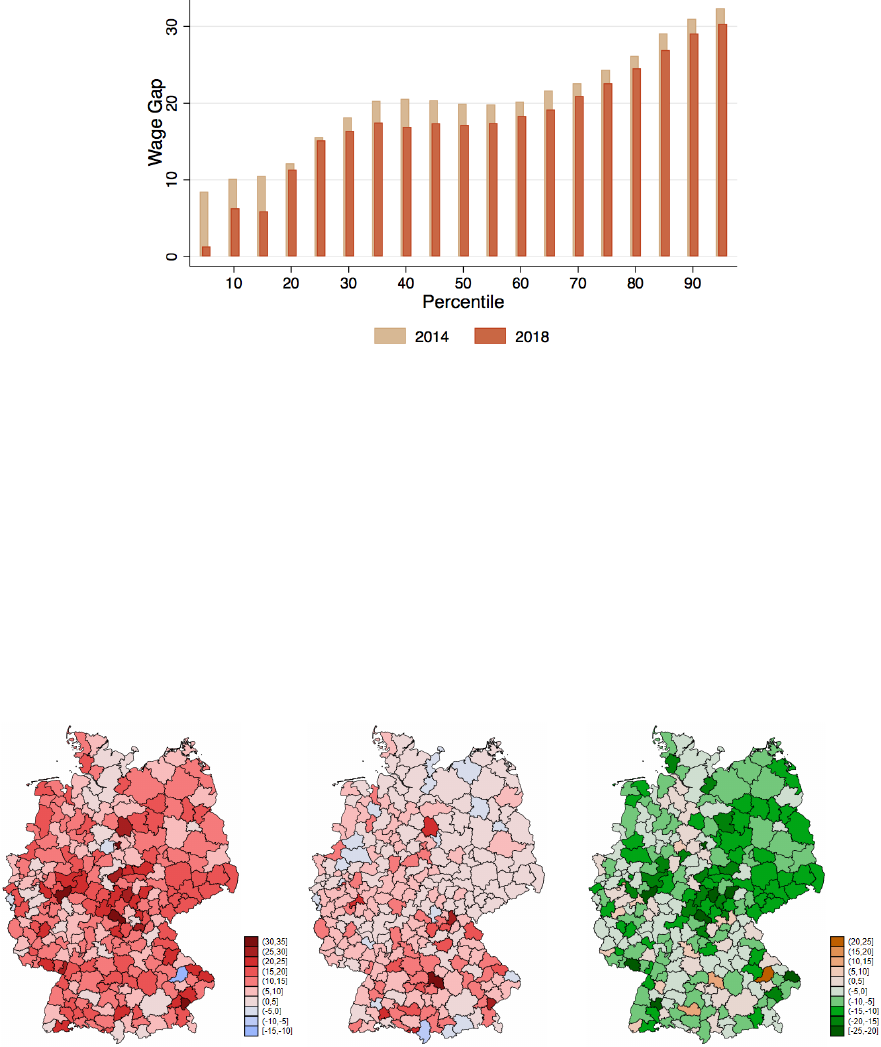
Figure 2: Wage Gaps at Percentiles of the Gender-speciﬁc Wage Distr i b ut i on, in %

Source: SES 2014 and 2018, own calculation. Includes only emp loyees eligibl e to the minimum wage, without

public sector personnel.

Figure 3: Regional Wage Gap at 10

percentile in 2014 and 2018 and Di↵erence in Gaps

between both Years (in Labour Market Regions)

(a) Gap in 2014 (in %) (b) Gap in 2018 (in %) (c) Di↵erence (in p.p.)

Source: SES 2014 and 2018 and BKG (2021), own calculat io n s . Note: Due to clearing restrictions, data for

Saxon regions is averaged for whole Saxony.

Figure 4: Fraction of A↵ected Female Employees in 2014 (in Labour Market Regi ons )

(a) Continu ous (in %) (b) Binary

Source: SES 2014 and BKG (2021), own calcula ti o n . Note: Due to clearing restrictions, data fo r Saxon regions

is averaged for whole Saxony.

Tables

Table 1: Descriptive Statistics on Wages, 2014 and 2018

2014 2018

All Men Women

Gap

All Men Women

Gap

(%) (%)

Share earning

<8.50 (%) 12.66 9.34 16.28 0.69 0.62 0.76

<8.84 (%) 15.47 11.54 19.76 2.83 2.39 3.33

Mean 16.80 19.03 14.36 24.54 18.71 20.86 16.29 21.91

SD 11.56 13.75 7.86 12.98 15.65 8.46

p10 8.01 8.56 7.70 10.05 9.46 9.82 9.21 6.21

p25 10.00 11.01 9.29 15.62 11.18 12.21 10.36 15.15

p50 14.11 15.67 12.54 19.97 15.58 17.10 14.17 17.13

p90 28.62 33.23 22.93 31.00 31.38 36.06 25.58 29.06

N755,431407,894347,537742,716409,571333,145

Source: SES 2014 and 20 1 8 , own calculations.

Note: We only includ e eligible employees that are not emp l oyed in the public service. The use d waves inclu d e

employees from sectors A to S from the WZ 2008 classiﬁcation. The SES contains workers t h a t a re em p loyed

throughout the whole month of April of the respective wave, but does not entail employees who are not paid

for the full month because they were newly hired or let go.

Table 2: Fixed E↵e ct s Re gre s si ons of Wage Gaps at 10

Percentile, 25

Percentile and Mean

(in Labour Market Regions)

(1) (2) (3) (4) (5) (6)

A: Wage Gap at p10

Bite x 2018 -5.228*** -5.085*** -4.870*** -4.735*** -4.550*** -4.550***

2018 -3.568*** -4.286*** -4.539*** -5.419*** -3.684 -3.754

GDP per capita (t-1) 0.153 0.152 0.126 0.147 0.158

Pop. Density (t-1) 0.024 0.020 0.017 0.015

Share of Women (t-1) -2.722 -2.837 -2.610

Empl. Rate Women (t-1) -0.412 -0.457

Childcare 0-2 (t-1) 0.044

Childcare 3-5 (t-1) -0.061

B: Wage Gap at p25

Bite x 2018 -3.352*** -2.814*** -3.122*** -3.111*** -3.191*** -3.336***

2018 -1.454** -4.154*** -3.792*** -3.865** -4.612 -4.079

GDP per capita (t-1) 0.576** 0.578** 0.576** 0.567** 0.541**

Pop. Density (t-1) -0.034 -0.034 -0.033 -0.027

Share of Women (t-1) -0.225 -0.176 0.010

Empl. Rate Women (t-1) 0.178 0.280

Childcare 0-2 (t-1) -0.239

Childcare 3-5 (t-1) 0.048

C: Wage Gap at Mean

Bite x 2018 -1.609* -1.339 -1.634* -1.684* -2.139** -2.297**

2018 -2.154*** -3.511*** -3.163*** -2.838* -7.110** -6.581**

GDP per capita (t-1) 0.289 0.292 0.301 0.249 0.229

Pop. Density (t-1) -0.032 -0.031 -0.023 -0.018

Share of Women (t-1) 1.006 1.289 1.662

Empl. Rate Women (t-1) 1.014* 1.092*

Childcare 0-2 (t-1) -0.228

Childcare 3-5 (t-1) 0.007

Observations 514 514 514 514 514 514

Groups 257 257 257 257 257 257

Source: SES 2014 and 20 1 8 , INKAR; own calculations.

Note:

⇤

p < 0.1,

⇤⇤

p < 0.05,

⇤⇤⇤

p < 0.01. The table displays the results of ﬁ x ed - e↵ec ts estimations in a

di↵erence-in-di↵erence framework with region-ﬁxed e↵ects and robust standard errors. The minimum wage

bite is binary and the regions are the 257 Labour Market Regions. In Panel A the dependent variable is the

unadjusted wage gap at the 10

percentile of the region a l gender-speciﬁc wage distribution. Accordingly, in

Panel B (C) the dependent variable is th e gap at the 25

percentile (the mean). The reference year is 2014.

Table 3: Fixe d E↵ects Regressions of Wage Gaps at 10

Percentile, 25

Percentile and Mean,

with Subsample, from 2010 to 2014 and 2014 to 2018 (in Labour Market Regions)

2010-2014 2014-2018

p10 p25 Mean p10 p25 Mean

(1) (2) (3) (4) (5) (6)

Bite x 2014 2.277 2.031 1.075

2014 -2.523 1.376 2.973

Bite x 2018 -4.947*** -2.831** -1.242

2018 -0.236 -2.608 -5.149

GDP per capita (t-1) 0.353 0.075 0.372 -0.130 0.374 0.011

Pop. Density (t-1) 0.013 0.031 -0.010 -0.006 -0.026 -0.025

Share of Women (t-1) 0.578 0.197 1.019 -1.377 4.160 2.737

Empl. Rate Women (t-1) 0.050 -0.016 -0.627 -0.171 0.352 1.027*

Childcare 0-2 (t-1) -0.169 -0.244 -0.337 -0.074 -0.249 -0.098

Childcare 3-5 (t-1) 0.246 -0.047 0.119 -0.013 0.038 0.014

Observations 514 514 514 514 514 514

Groups 257 257 257 257 257 257

Source: SES 2014 and 20 1 8 , INKAR; own calculations.

Note:

⇤

p < 0.1,

⇤⇤

p < 0.05,

⇤⇤⇤

p < 0.01. The table displays the results of ﬁ x ed - e↵ec ts estimations in a

di↵erence-in-di↵erence framework with region-ﬁxed e↵ects and robust standard errors. The minimum wage

bite is binary and the regions are the 25 7 Labour Market Regions. Colu mn s (1)-(3) include regressions entailing

the years 2010 and 2014, Co l u mn s (4)-(6) show regressions containing the years 2014 and 2018. In Columns

(1) and (4) the dependent va ri a b le is the unadju st ed wage g a p at the 10

percentile of the regional gender-

speciﬁc wage distribution. Accordingly, in Columns (2 ) and (5) the dependent variable is the gap at the 25

percentile, in Columns (3) and (6) it is the gap at the mean. The reference year is 2010 for Columns (1)-(3)

and 2014 for Columns (4)-(6). The subsample is identiﬁed via the variab le GG2010, which is provided by the

federal statistical o ﬃc e and which adapts the 2014 and 2018 data to the structure of t h e 2010 wave (FDZ der

Statistischen

Amter des Bundes und der L¨ander, 2019).

Appendix

Table A.1: Descriptive Statistics on Wages of Subsample 2010-2018

2010 2014 2018

Men Women

Gap

Men Women

Gap

Men Women

Gap

(%) (%) (%)

Share earning

<8.50 (%) 9.95 19.44 6.25 11.85 0.54 0.71

<8.84 (%) 11.34 22.02 7.91 14.65 1.76 2.62

Mean 19.16 14.43 24.67 20.54 15.64 23.88 22.35 17.55 21.50

SD 12.84 7.67 14.33 8.45 16.48 9.19

p10 8.50 7.48 11.95 9.26 8.20 11.50 10.30 9.55 7.28

p25 11.65 9.21 20.94 12.36 9.94 19.58 13.41 11.14 16.93

p50 16.20 13.13 18.96 17.24 14.02 18.71 18.56 15.53 16.32

p90 32.65 22.75 30.32 35.17 24.82 29.44 38.29 27.68 27.70

N892,994612,996345,701265,859328,844244,403

Source: SES 2010, 2014 a n d 2018, own calculations.

Note: We only inclu d e eligi b le employees that are not employed in the public service. The subsample is

identiﬁed via the variable GG2010, which is p rovided by the federal statistical oﬃce and which adapts the

2014 and 2018 data to the structure of the 2010 wave (FDZ der Statistischen

Amter des Bundes und der

L¨ander, 2019).

Table A.2: Sensitivity Analyses: Fixed E↵ects Regressions of Wage Gaps at 10

Percentile,

Percentile and Mean

A: Main Results B: Bite for All C: Continuous Bite

p10 p25 Mean p10 p25 Mean p10 p25 Mean

Bite x 2018 -4.550*** -3.336*** -2.297** -2.617*** -2.272** -1.792* -0.333*** -0.277*** -0.183***

2018 -3.754 -4.079 -6.581** -4.000 -4.084 -6.471** 2.016 0.877 -3.336

Controls yes yes yes yes yes yes yes yes yes

Observations 514 514 514 514 514 514 514 514 514

Groups 257 257 257 257 257 257 257 257 257

D: No MW Sectors E: ROR F: Districts

p10 p25 Mean p10 p25 Mean p10 p25 Mean

Bite x 2018 -4.207*** -3.051** -3.323*** -3.730*** -2.185* 0.133 -3.951*** -3.196*** -1.286*

2018 -3.598 -6.162* -7.601** -1.881 0.113 0.461 -0.739 -3.612 -3.275

Controls yes yes yes yes yes yes yes yes yes

Observations 514 514 514 192 192 192 802 802 802

Groups 257 257 257 96 96 96 401 401 401

G: No Individual Weights H: Regression Weights

p10 p25 Mean p10 p25 Mean

Bite x 2018 -4.577*** -2.267** -1.466* -4.868*** -2.828*** -1.413*

2018 -3.597* -2.361 -4.486* -0.782 -0.362 -2.578

Controls yes yes yes yes yes yes

Observations 514 514 514 514 514 514

Groups 257 257 257 257 257 257

Source: SES 2014 and 20 1 8 , INKAR; own calculations.

Note:

⇤

p < 0.1,

⇤⇤

p < 0.05,

⇤⇤⇤

p < 0.01. The table displays the results of ﬁ x ed - e↵ec ts estimations in a

di↵erence-in-di↵erence framework with region- ﬁ xed e↵ects and robust standard erro rs . Control variables are

included as in Table 2 but not reported. In the ﬁrst column of each panel the dependent variable is the

unadjusted wage gap at the 10

percentile of the region a l gender-speciﬁc wage distribution. Accordingly, in

the second (third) column the dep en d ent variable is the gap at the 25

percentile (the mean). The reference

year for all estimations is 20 1 4 . We adapt them main speciﬁcation as follows: In Panel A we display the main

results from Ta b le 2 for comparison. In Panel B employ the minimum wage bite for all employees, irrespective

of their gender. In Panel C we use a continuous fraction rather than a binary one. In Panel D we exclude

individuals working in sectors with sector-speciﬁc minimum wage agreements. Panel E and F do not rely on

Labour Market Regions but Planning Regions (E) and Districts (F). In Panel G we do not use individual

weights for calculating the bite and the regional wage distribution. In Panel H we weight the regions in the

regression using the absolute regional employment as weights.